hsl and hsv
hsl and hsv are two widely used color models that align more closely with human vision perception of colors; their use can be found in imaging software, camera tools, web standards, and many other applications; there are simple formulas to convert between rgb and hsl/hsv color models, yet very few documents explaining the mathematics behind those formulas in full details; so, this article aims to be a comprehensive description of these models and conversions between relative color models;
motivation
why did people invent hsl and hsv color models? where does rgb color model fall
short? imagine you are drawing a picture with a blue-ish color #0080ff; after
some review you would like to adjust its lightness and fullness, while keep the
same blue-ish; if you are not a color expert, you get frustrated with the color
slides of rgb components because when you change them the color no longer looks
the same as before; when you start using hsl/hsv color models, this job becomes
much easier: you can fix hue and adjust saturation and lightness/value, which
gives a variety of colors, all having the same blue-ish as before; this is an
example of more intuitive color picking and mixing;
background
the discussion below is slightly complicated so we need some background as well
as convention; first, we let each rgb component be a float in range [0.0, 1.0]
and assume computation has arbitrary precision; second, we order rgb components
as (R, G, B); third, we arrange rgb gamut in a unit cube, within a coordinate
system where black is at origin and white is at (1.0, 1.0, 1.0) unless we use
an alternative coordinate system; fourth, we denote the vertices of the cube by
a single letter as such: black(K), red(R), green(G), blue(B), cyan(C),
magenta(M), yellow(Y), white(W); fifth, we will discuss hsv before hsl as
we feel hsv formula is easier to derive and understand; sixth, we omit a corner
case (eg: divide by zero) at various places where it simplifies analysis so you
are advised to compare this article against the wikipedia article
for completeness;
hsv
hsv stands for hue, saturation, value:
-
hue gives the “tone” of the color (eg: reddish, yellowish, etc.);
-
saturation gives the “fullness” of the color; high saturation feels vibrant while low saturation feels pale;
-
value gives the “brightness” of the color; this is the amount of maximum component (will be defined soon);
look at these pictures to understand how they vary:
 |
 |
the left picture is an intermediary result (hue-chroma-value, hcv); the right picture is the final result (hue-saturation-value, hsv); as you can see, hsv arranges colors in a cylinder; as we will see, this cylinder can be converted from the rgb unit cube, with the hcv cone as an intermediary result (video);
hue and chroma
now we mathematically define the hue in hsv; we first define chroma; chroma is a value of “colorfulness” and it is closely related to saturation;
assume we have rgb color \((R, G, B)\); we define:
-
maximum component \(M_2=M=\text{max}(R, G, B)\);
-
minimum component \(M_0=m=\text{min}(R, G, B)\);
-
middle component \(M_1\) as the component other than \(M_2\) and \(M_0\);
-
chroma \(C=M_2-M_0\);
-
hue offset \(H’’ =(M_1-M_0)/(M_2-M_0)\); \(H’’ =0\) if \(M_2=M_0\);
differences from wikipedia:
-
wikipedia uses two symbols \(M\) and \(m\), we use three symbols \(M_2\), \(M_1\) and \(M_0\) because we need an explicit middle component;
-
wikipedia uses a piecewise definition for hue, we use a concise formula to compute hue offset; this formula works in all pieces; later on, we will compute hue using hue offset;
-
wikipedia defines \(H=60^{\circ} \times H’\), we do not distinct \(H\) from \(H’\) because they are essentially the same thing, only with different units and ranges;
the picture below visualizes these definitions:
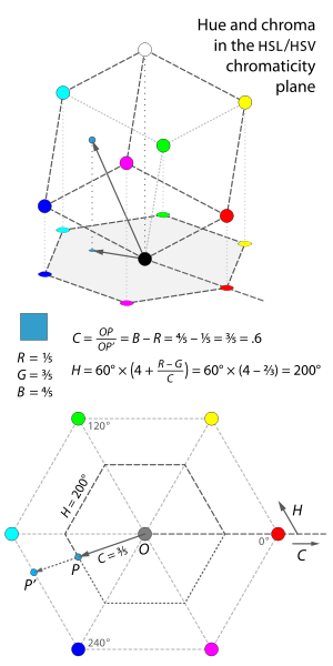
this is a very important picture showing the rgb-to-hsv conversion; we first
tilt the rgb unit cube so that black is at origin and white is vertically above
it; then we project it onto a “chromaticity plane” perpendicular to the
black-white axis; the projection is a hexagon as shown; why is it a hexagon? it
is easily seen from symmetry that R, G, B form an equilateral triangle; so
do C, M, Y; and ROC, GOM, BOY are collinear;
this picture gives intuition about the definitions of chroma and hue:
-
chroma is the proportion of the distance from the origin to the edge of the hexagon; it is the same as the ratio of the radii of the two hexagons;
think chroma as “magnitude”;
-
hue is roughly the angle we walk counterclockwise from red (\(0^{\circ}\)) to the point; “roughly” means there is a very small error introduced by chords and arcs, as we shall see;
think hue as “phase”;
this picture shows an interesting property: adding or subtracting the same amount from all three of R, G, B components does not change its projection, and thus does not change chroma or hue; that is, given any point in the cube, we can always move it down vertically until it lies on one of the three lower faces of the cube; all points on these faces have at least one zero component;
this picture shows another interesting property: the projection is divided
evenly into 6 areas (quadrants, but for 6, or sextants): ORY (area 0), OYG
(area 1), OGC (area 2), OCB (area 3), OBM (area 4), OMR (area 5); in
each area, the order of R, G, B components are uniquely determined; for example,
if a point has its projection in area OCB, then we know \(B \ge G \ge R\):
-
when we move it vertically down, we are subtracting the same amount from all three components; then it crossed face
OGB, which means red component came to zero first, so the red component is the smallest; -
its projection is closer to blue than green, so the point on face
OGBmust have a larger blue component than green component; adding the same amount of red, green and blue maintains this comparison result;
finally we can start computing chroma and hue; let the point be \((R, G, B)\);
wlog we assume it is an area 3 (OCB) point; from the above observations, we
know \(B \ge G \ge R\); so we can use point Q at \((0, G-R, B-R)\) to
compute the same chroma and hue; we know Q lies on cube face OGB;
-
to compute chroma \(C\), we extend
OQto intersect segmentBCat a pointQ'; we knowOP/OP' = OQ/OQ'becauseQPis parallel toQ'P'; if we projectQandQ'onto edgeOBat pointsTandT'respectively, then we knowOQ/OQ' = OT/OT'; butT'is exactlyB,OT'has length \(1\), andOThas length \(B-R\) (blue component ofQ); so \(C=B-R=M_2-M_0\);do this in other areas and you will find \(C=M_2-M_0\) always holds;
-
to compute hue, we first compute hue offset \(H’’\); the hue offset measures how far the input point is away from its closest primary vertex; there are three primary vertices
R,G,B; when input point is in area 3, its closest primary vertex isB; so the hue offset isBP'/BC=BQ'/BC(BandCin the right hand side refer to vertices in the cube, not the plane); becauseBis \((0, 0, 1)\),Cis \((0, 1, 1)\),Q'is \((0, (G-R)/(B-R), 1)\) (computed fromQ), we haveto compute hue from hue offset, we first notice the point lies in area 3, so the closest primary vertex is
Band we should go clockwise (subtract); now we subtract hue offset from the angle ofB(\(240^{\circ}\), or \(4\) sextants); in this example, \(H’’ =2/3\), so we compute hue as \(H=(4-2/3) \times 60^{\circ}=200^{\circ}\); the hue offset captures the amount of middle component relative to maximum component (with pure white light removed); and you can verify our hue computed from hue offset matches the wikipedia piecewise function in every piece;finally, our computation here is based on a hexagon not a circle; and the hue offset is a ratio of chords not arcs; for the hsv color space to be a cylinder, an additional warping that maps linearly each chord into an arc turns the hexagon into a circle; this still maps a hsv tuple to the same color, but only changes the shape of the hsv color space; we will omit this detail afterwards;
value
the definition of value in hsv is very simple: it is the value of maximum component:
- value \(V=M_2\);
for example, for a blue-ish color (blue is the maximum component), value tells how much blue there is in it;
this definition gives a “hexcone” model: all three primary colors RGB, all
three secondary colors CMY, and white color W are placed in a plane at the
top of tilted cube; visually, this transformation is like opening an umbrella
from top to bottom; or you can think the cube as an onion with its core at the
black origin K and is peeled layer by layer from top to bottom, with each
layer composed by three quadrants perpendicular to each other;
saturation
saturation is closely related to chroma \(C\):
- saturation \(S=C/V\);
this means saturation is chroma scaled into range [0.0, 1.0]; to see this,
recall \(C=M_2-M_0\) and \(V=M_2\), so \(0 \le C \le V\); dividing \(C\)
by \(V\) does the scale; the corner case is when \(V=0\), then \(S\) is
defined trivially as \(0\);
replacing chroma with saturation expands the bottom of the hexcone to turn into a cylinder;
hsv to rgb
here we have finished the conversion from rgb to hsv; now we talk about the other direction: hsv to rgb;
the hsv-to-rgb conversion steps are:
-
compute \(C=V \times S\); then \(M_2-M_0=C\);
-
compute \(M_2=V\); then \(M_0=V-C\);
-
compute hue offset \(H’’\); this computation can be done by looking at the chromaticity plane to decide which of
R,G,Bis the closest primary vertex: useRif area 0 or 5,Gif area 1 or 2,Bif area 3 or 4; then the computation of \(H’’\) is simply an addition or subtraction of \(H\) and the angle of the primary vertex;once we have \(H’’ =(M_1-M_0)/(M_2-M_0)\), we can compute \(M_1\);
-
now we have all three components; use \(H\) to find their order (ie: map \(\{M_0,M_1,M_2\}\) to \(\{R, G, B\}\));
hsv to rgb (optimized)
the above algorithm is easy to comprehend, but may not be the best for machines to run; to develop an optimized algorithm for machines, we observe this fact: for fixed \(S\) and \(V\) and varying \(H\), each RGB component range is limited to \([V-VS, V]\); to see this, let us take green component as an example:
-
when area is 4 or 5, green component is the minimum component \(M_0\), so it is equal to \(M_2-(M_2-M_0)=V-C=V-VS\);
-
when area is 1 or 2, green component is the maximum component \(M_2\), so it is equal to \(V\);
-
when area is 0 or 3, green component is the middle component \(M_1\), so it is between \(M_0\) and \(M_2\), that is, in range \([V-VS, V]\);
in this case there is one more observation: \(H’’\) is linear in \(M_1\) because \(M_0\) and \(M_2\) are fixed, so \(H\) is linear in \(M_1\) because \(H’’\) and \(H\) only differ by a constant; adjacent areas are obviously continuous (when \(H\) is gradually increased, the point moves continuously), so we can connect the endpoints of its two adjacent areas with a straight line (area 2 and 4 for area 3, area 5 and 1 for area 0);
now we get a function mapping \(H\) to green component \(G\) which has a flat top, a flat bottom, and two slopes; it looks like this (green line):

this function can be realized with clever use of \(\min\) and \(\max\); someone has worked it out as (plot):
as you can see, red, green, blue components work in the same way, only with different shifts;
hsl
hsl stands for hue, saturation, lightness:
-
hue gives the “tone” of the color (eg: reddish, yellowish, etc.);
-
saturation gives the “fullness” of the color; high saturation feels vibrant while low saturation feels pale; note that saturation in hsv and hsl have a similar meaning but are computed differently: saturation is chroma divided by max chroma in both hsv and hsl, but that max chroma (ie: divisor) is value in hsv, and a function on lightness in hsl; where necessary, we use \(S_V\) for saturation in hsv, and \(S_L\) for saturation in hsl;
-
lightness gives the “lightness” of the color; its difference from value in hsv is that, value takes the amount of one component (maximum component), while lightness takes the average of two (maximum and minimum components);
look at these pictures to understand how they vary:
 |
 |
the left picture is an intermediary result (hue-chroma-lightness, hcl); the right picture is the final result (hue-saturation-lightness, hsl); as you can see, hsl arranges colors in a cylinder; as we will see, this cylinder can be converted from the rgb unit cube, with the hcl bicone as an intermediary result (video);
hue and chroma
hue and chroma in hsl are defined exactly the same as in hsv;
lightness
the definition of lightness in hsl is the average of maximum and minimum components:
- lightness \(L=(M_2+M_0)/2\);
this definition gives a “bi-hexcone” model: all three primary colors RGB, all
three secondary colors CMY, and white color W are placed in a plane at the
half of tilted cube; if you divide the cube into many tiny cubes arranged in
three dimensions, and calculate lightness of the outermost ones (the ones on its
six faces), you will find the amount of lightness is a pyramid in the three
upper faces, and an inverted pyramid in the three lower faces; when you strip
these tiny cubes on the surface, you are left with a smaller tilted cube
possessing a similar structure (eg: \((255, 0, 0)\) becomes \((254, 1, 1)\),
\((255, 0, 255)\) becomes \((254, 1, 254)\), etc.); since \(255+0=254+1\),
the six corners RGBCMY of the smaller cube are on the same plane as those on
the original cube; this suggests the bi-hexcone is pretty much like our earth:
RGBCMY are aligned on the equator, white is the north pole and black is the
south pole;
saturation
saturation is closely related to chroma \(C\):
- saturation \(S=C/(1-|2L-1|)=C/(2\min(L,1-L))\);
this means saturation is chroma scaled into range [0.0, 1.0]; to see this,
recall \(C=M_2-M_0\) and \(L=(M_2+M_0)/2\); the lower bound of \(C\) is
\(0\) (equal when \(M_2=M_0\)); the upper bound of \(C\) is \(2L\)
if \(2L \le 1\) (equal when \(M_0=0, M_2=2L\)), or \(2-2L\) if
\(2L \ge 1\) (equal when \(M_0=2L-1, M_2=1\));
the corner case is when \(L=0\) or \(L=1\), then \(S\) is defined trivially as \(0\);
replacing chroma with saturation expands the top and bottom of the bi-hexcone to turn into a cylinder;
hsl to rgb
here we have finished the conversion from rgb to hsl; now we talk about the other direction: hsl to rgb;
the hsl-to-rgb conversion steps are:
-
compute \(C=2\min(L,1-L) \times S\); then \(M_2-M_0=C\);
-
we know \(M_2+M_0=2L\); so \(M_2=L+C/2\) and \(M_0=L-C/2\);
-
compute hue offset \(H’’\); this computation can be done by looking at the chromaticity plane to decide which of
R,G,Bis the closest primary vertex: useRif area 0 or 5,Gif area 1 or 2,Bif area 3 or 4; then the computation of \(H’’\) is simply an addition or subtraction of \(H\) and the angle of the primary vertex;once we have \(H’’ =(M_1-M_0)/(M_2-M_0)\), we can compute \(M_1\);
-
now we have all three components; use \(H\) to find their order (ie: map \(\{M_0,M_1,M_2\}\) to \(\{R, G, B\}\));
hsl to rgb (optimized)
the above algorithm is easy to comprehend, but may not be the best for machines to run; to develop an optimized algorithm for machines, we observe this fact: for fixed \(S\) and \(L\) and varying \(H\), each RGB component range is limited to \([L-C/2, L+C/2]\) (\(C\) can be computed using only \(S\) and \(L\)); to see this, let us take green component as an example:
-
when area is 4 or 5, green component is the minimum component \(M_0\), so it is equal to \(M_0=L-C/2\);
-
when area is 1 or 2, green component is the maximum component \(M_2\), so it is equal to \(M_2=L+C/2\);
-
when area is 0 or 3, green component is the middle component \(M_1\), so it is between \(M_0\) and \(M_2\), that is, in range \([L-C/2,L+C/2]\);
in this case there is one more observation: \(H’’\) is linear in \(M_1\) because \(M_0\) and \(M_2\) are fixed, so \(H\) is linear in \(M_1\) because \(H’’\) and \(H\) only differ by a constant; adjacent areas are obviously continuous (when \(H\) is gradually increased, the point moves continuously), so we can connect the endpoints of its two adjacent areas with a straight line (area 2 and 4 for area 3, area 5 and 1 for area 0);
now we get a function mapping \(H\) to green component \(G\) which has a flat top, a flat bottom, and two slopes; it looks quite similar to the one in hsv above, but wikipedia does not give a plot for hsl;
this function can be realized with clever use of \(\min\) and \(\max\); someone has worked it out as (plot):
as you can see, red, green, blue components work in the same way, only with different shifts;
interconversion
interconversions between hsv and hsl can be computed directly without using rgb; we will be using these facts for the interconversions:
hsv to hsl
to compute \(\{H_L, S_L, L\}\) from \(\{H_V, S_V, V\}\):
hsl to hsv
to compute \(\{H_V, S_V, V\}\) from \(\{H_L, S_L, L\}\):
3d visualization
here are amazing 3d visualizations of hsl and hsv color models, coming from a bachelor thesis; you can play with them interactively to see how the point moves simultaneously in the rgb cube and in the cone/bi-cone;
epilog
some of you might get disappointed, sadly, there are no snippets for conversion between rgb and hsl/hsv in this article; the reason is i do not want to present a possibly flawed implementation that could misbehave in production, and i have no idea what programming language you will be using; so just search online, for a mature library in your language;
another thing good to mention here is units and ranges; everything works fine
without units and with values in range [0.0, 1.0], since this is merely a
geometric transformation; however, you will typically see in software, hue in
range [0, 360], value, lightness, saturation in range [0, 100]; the hue is
in degree, all others are in percentage; these units and ranges are for
convenience reasons;
it is probably good to end this article with this picture:

references
- https://en.wikipedia.org/wiki/File:HSL-HSV_hue_and_chroma.svg
- https://en.wikipedia.org/wiki/File:HSL_color_solid_cylinder_saturation_gray.png
- https://en.wikipedia.org/wiki/File:HSL_color_solid_dblcone_chroma_gray.png
- https://en.wikipedia.org/wiki/File:HSV-RGB-comparison.svg
- https://en.wikipedia.org/wiki/File:HSV_color_solid_cone_chroma_gray.png
- https://en.wikipedia.org/wiki/File:HSV_color_solid_cylinder_saturation_gray.png
- https://en.wikipedia.org/wiki/File:Hsl-and-hsv.svg
- https://en.wikipedia.org/wiki/File:RGB_2_HSL_conversion_with_grid.ogg
- https://en.wikipedia.org/wiki/File:RGB_2_HSV_conversion_with_grid.ogg